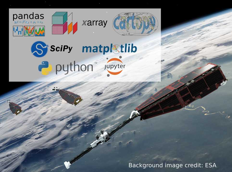
viresclient: Programmatic access to Swarm
ashley.smith@ed.ac.uk ... View slides: https://bit.ly/2lYAuQm
![]()
Aims
Direct access to "computation-ready" data without worrying about:
- file formats; file organisation
- model forward code
Provide a dependable interface to a wide arrange of "data"
- new products added / old products changed: access them in the same way
Complementary to the VirES web interface
- More prerequisite knowledge needed (++time)
- ... but more freedom than the GUI
1: Basic usage: accessing data
In [2]:
from viresclient import SwarmRequest

request = SwarmRequest()
request.set_collection("SW_OPER_MAGA_LR_1B")
request.set_products(["F", "B_NEC"])
data = request.get_between("2019-01-01", "2019-01-02")
print(data)
In [3]:
data.to_file("test_file.cdf", overwrite=True)
2: Basic usage: translating to a Pandas dataframe
In [4]:
df = data.as_dataframe(expand=True)
df.head()
Out[4]:
In [5]:
%matplotlib inline
df["F"].plot();

Some very short Pandas examples....
In [6]:
df.describe()
Out[6]:
In [7]:
from pandas.plotting import autocorrelation_plot

df["F"].resample("60s").mean().pipe(autocorrelation_plot);

You can still directly access Numpy arrays from a dataframe:
In [8]:
df[["B_NEC_N", "B_NEC_E", "B_NEC_C"]].values
Out[8]:
3. Basic usage: translate to an xarray Dataset

In [9]:
ds = data.as_xarray()
ds
Out[9]:
In [10]:
ds["B_NEC"].plot.line(figsize=(10,5), x="Timestamp");

4. Robust and easy access to larger volumes of data and models
In [11]:
request = SwarmRequest()
request.set_collection("SW_OPER_MAGA_LR_1B")
request.set_products(
    measurements=["B_NEC"], models=["CHAOS-6-Core"], residuals=True,
    auxiliaries=["MLT", "QDLat"], sampling_step="PT60S")
request.set_range_filter("Flags_F", 0, 1)
data = request.get_between("2019-01-01", "2019-07-01")  # 6 MONTHS

df = data.as_dataframe(expand=True)
df.plot(y="B_NEC_res_CHAOS-6-Core_C", x="QDLat", kind="scatter", figsize=(10,3),
        c="MLT", cmap=cm.RdYlBu, s=1, alpha=0.5);

Names of original data files are logged
In [12]:
data.sources[-10:]
Out[12]:
"One-line" analysis
In [13]:
ds = data.as_xarray()
fig, ax = plt.subplots(1, 1, figsize=(10, 2))
(ds.groupby_bins("QDLat", 90)
   .apply(lambda x: x["B_NEC_res_CHAOS-6-Core"].std(axis=0))
   .plot.line(x="QDLat_bins", ax=ax)
)
ax.set_title("Standard deviations");

Want to do this? Learn Pandas & Xarray (& Numpy & Matplotlib)
Want to scale it to larger data? Learn Dask.
In [15]:
from viresclient import SwarmRequest
import matplotlib.pyplot as plt
from matplotlib.dates import DateFormatter

request = SwarmRequest()
request.set_collection("SW_OPER_IPDAIRR_2F")
request.set_products(measurements=request.available_measurements("IPD"))
data = request.get_between("2014-12-21T00:00", "2014-12-21T03:00")
df = data.as_dataframe()

fig, axes = plt.subplots(nrows=7, ncols=1, figsize=(20,11), sharex=True)
df.plot(ax=axes[0], y=['Background_Ne', 'Foreground_Ne', 'Ne'], alpha=0.8)
df.plot(ax=axes[1], y=['Grad_Ne_at_100km', 'Grad_Ne_at_50km', 'Grad_Ne_at_20km'])
df.plot(ax=axes[2], y=['RODI10s', 'RODI20s'])
df.plot(ax=axes[3], y=['ROD'])
df.plot(ax=axes[4], y=['mROT'])
df.plot(ax=axes[5], y=['delta_Ne10s', 'delta_Ne20s', 'delta_Ne40s'])
df.plot(ax=axes[6], y=['mROTI20s', 'mROTI10s'])
for ax in axes:
    ax.xaxis.set_major_formatter(DateFormatter("%Y-%m-%d\n%H:%M:%S"))
    ax.legend(loc="upper right")
    ax.grid()
fig.subplots_adjust(hspace=0)
plt.close()
Replace the previous with:
from viresclient import SwarmQuicklook
fig = SwarmQuicklook("IPDxIRR", spacecraft="Alpha", options...)
In [16]:
fig
Out[16]:

6. Future development: integrate with other libraries
 |
 |
 |
| PyViz advanced visualisation: |  |
| Domain-specific libraries: |  |
 |
 |
? Swarm-DISC... |
In [17]:
import hvplot.pandas
df.hvplot(y=['Background_Ne', 'Foreground_Ne', 'Ne'])
Out[17]:
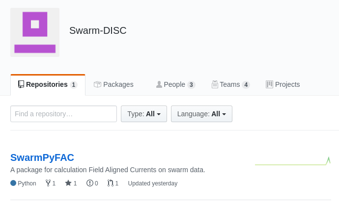
7. Develop other packages which connect to viresclient
SwarmPyFAC (author: Ask Neve Gamby)
New Swarm-DISC GitHub organisation
https://github.com/Swarm-DISC/SwarmPyFAC
In [19]:
import swarmpyfac as fc
import datetime as dt
import numpy as np
import matplotlib.pyplot as plt
%matplotlib inline
output, input_data = fc.fac_from_file(start=dt.datetime(2016, 1, 1), end=dt.datetime(2016, 1, 2), user_file=None)
time, position, __, fac, *___ = output
selection = np.arange(380,3000)
fig, axes = plt.subplots(nrows=1, ncols=2, figsize=(15,5))
axes[0].plot(time,position[:,0],'b')
axes[0].plot(time[selection],position[selection,0],'r')
axes[0].set_xlabel('time [s]]'); axes[0].set_ylabel('latitude [degree]')
axes[1].plot(position[selection,0],fac[selection],'b')
axes[1].set_xlabel('latitude [degree]'); axes[1].set_ylabel('$J_{||} \; [nA/m^2]$')
axes[1].axis([-90, 90, -15,15]);

8. Compatibility and versioning
- viresclient defines a general purpose data access layer for other packages to depend on
- Semantic versioning. Read this if you are producing a package: https://semver.org
In [20]:
import viresclient
viresclient.__version__
Out[20]:
- Forwards compatibility is a priority but can't be guaranteed right now - check the change log
- Aim to formalise interface and move to a 1.0 release when appropriate
Summary
- viresclient: https://viresclient.readthedocs.io/en/latest/installation.html
- VRE: https://swarm-vre.readthedocs.io
- Ongoing development of viresclient tying the VirES/VRE services together
- Aim to integrate with other Python packages
- General Python software (many 1000's of contributors)
- Swarm software from the community: Coordinate using GitHub (see e.g. sunpy)
- Need feedback and feature requests for real use cases
- Need community-led development of packages
- Use cases:
- from rapid development, to producing repeatable & portable analyses
- data access layer for other affiliated packages (Swarm-DISC activities)
- integrating VirES with other services (e.g. Swarm-Aurora/AuroraX)